Anomaly Detection through Reinforcement Learning

As Artificial Intelligence is becoming a mainstream and easily available commercial technology, both organizations and criminals are trying to take full advantage of it. In particular, there are predictions by cyber security experts that going forward, the world will witness many AI-powered cyber attacks¹. This mandates the development of more sophisticated cyber defense systems using autonomous agents which are capable of generating and executing effective policies against such attacks, without human feedback in the loop.

In this series of blog posts, we plan to write about such next generation cyber defense systems. One effective approach of detecting many types of cyber threats is to treat it as an anomaly detection problem and use machine learning or signature-based approaches to build detection systems. Anomaly Detection Systems (ADS) are also used as the core engines powering authentication and fraud detection platforms, for applications such as continuous authentication which Zighra provides through its SensifyID platform.

Anomaly Detection using Machine Learning

Anomaly Detection Systems (ADS) are designed to find patterns in a dataset that do not conform to expected normal behavior. Most of the anomaly detection problems can be formulated as a typical classification task in machine learning, where a dataset containing labelled instances of normal behavior (also of abnormal behavior if data is available) is used for training a supervised or semi-supervised machine learning models such as neural networks or support vector machines². Though unsupervised learning also could be used for anomaly detection, they are shown to perform very poorly compared to supervised or semi-supervised learning³.

Since in domains such as cyber defensedefence, the attack scenarios change continuously due to constant evolution by the attackers to avoid detection systems, it is important to have a continuous learning system for anomaly detection. This could be achieved in principle using online learning where a continuous supervised signal (whether the past predictions were correct or not) is fed back into the system and the model is continuously trained with more weights given to recent data to incorporate concept shifts in the dataset.

However, there are many anomaly detection problems where a straightforward online learning is either not feasible or not good enough to provide highly accurate predictions. In such scenarios, one could formulate the anomaly detection problem as a reinforcement learning problem^4,5, where an autonomous agent interacts with the environment and takes actions (such as allowing or denying access) and gets rewards from the environment (positive rewards for correct predictions of anomaly and negative rewards for wrong predictions) and over a period of time learns to predict anomalies with a high level of accuracy. Reinforcement learning brings the full power of Artificial Intelligence to anomaly detection.

In this blog, we will describe how reinforcement learning could be used for anomaly detection giving an example of network intrusion through Bot attacks. To begin with, let us see how a reinforcement learning problem can be described in a mathematical framework called Markov Decision Process or MDP.

Reinforcement Learning in Nutshell

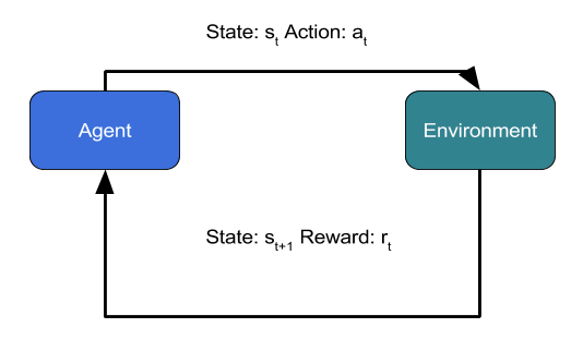
MDP is defined by a 5-Tuple consisting of State at time t (st), Action in state s (at), State Transition Probabilities P(st+1|st, at) , Discount factor for future Rewards (γ) and Reward function rt. The objective of MDP is to come up with an optimal policy Π* (what action should be taken at each state) so that the agent achieves maximum payoff (cumulative rewards) over a long period of time.

There are several approaches for solving a MDP problem. One of the well-known methods is called Q-Learning. Here one defines a Quality function Q(s, a) which gives an estimate of the maximum total reward or payoff the agent can receive starting from state s and performing action a. The value of Q(s, a) for all states and actions can be found through solving the Bellman equation:

Q(s, a) = r + γ maxa Q(s’, a’)

which states that the maximum total long term reward that one can obtain starting from state s and performing action a is the sum of current reward r plus the maximum total long term rewards that can be obtained from the next state s’ weighted by the discount factor γ. Bellman equation is the central theoretical concept that is used in almost all formulations of reinforcement learning. It can be proved that starting from random initial conditions, by repeatedly iterating the above equation, Q(s, a) will converge to an optimum Quality function Q*(s, a). Then the optimal policy is given by:

Π*(s) = argmaxa Q*(s, a)

In practice, a derivative form of the Bellman equation is used in many implementations. This is an iterative updating algorithm called the Temporal Difference Learning algorithm. Here, upon the agent making a transition from state s to state s’, the Q values are updated through the equation:

Q(s, a) = (1 – α ) Q(s, a) + α (r + γ maxa Q(s’, a’))

Here α is a parameter representing the learning rate.

Function Approximation using Neural Networks

When states are discrete and the number of possible states and actions are small, it is straightforward to use the above equation for finding optimum values of Q(s, a) and optimum policy Π*(s). However, in many practical scenarios, there are a very large number of states and the above approach would fail to scale. For example, consider the application of RL to play the game MsPacman. There are over 250 pellets that MsPacman can eat, each of which can be present or absent. Therefore, the total number of possible states is 2²⁵⁰ ~ 10⁷⁵. To avoid the curse of dimensionality problem, one tries to approximate Q-Values using a Deep Neural Network with a manageable number of parameters⁶. This can be conceptually represented by the following diagram:

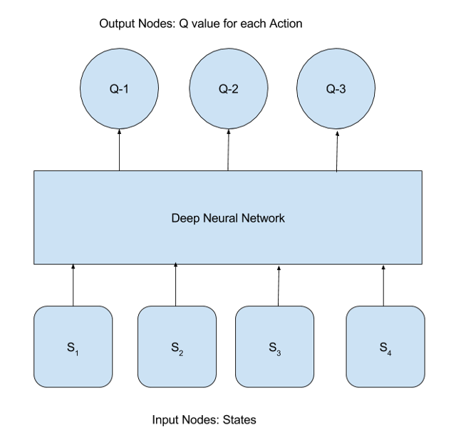
Here, input to the DNN are the states and the output, the Q-values for each action. The difference between the Q-values predicted by the DNN and the target Q values given by the Bellman equation is considered to be the error (or loss function) of prediction by the DNN:

L = ½ [ (r + γ maxa Q(s’, a’)) – Q(s,a) ]²

The Neural Network model is trained using the back propagation algorithm as follows:

1. Initialize Q(s, a) and start from a random state s
2. Do a forward pass of state s through the DNN and get Q-values for all actions
3. Perform an ε-greedy exploration for choosing an action a for the current state s. This is done by choosing a random action with a small probability ε, otherwise selecting the action having largest Q-value for state s.
4. Pass forward the next state s’, obtained after performing action a in step 3, also through the DNN and calculate the maximum overall network outputs, maxa Q(s’, a’)
5. Set the target Q-value for the output node corresponding to action a to be r + γ maxa Q(s’, a’). For all other nodes, keep the target Q-value same as that obtained from DNN prediction in step 2.
6. Update the weights using back propagation.
7. Repeat the steps 2-6 till the network is trained.

Once the DNN is trained after enough episodes of exploration by the agent interacting with the environment (usually of the order of 1000s of episodes), it can be used for selecting the best action for a given state which will produce maximum total rewards in a long time.

Network Intrusion Detection

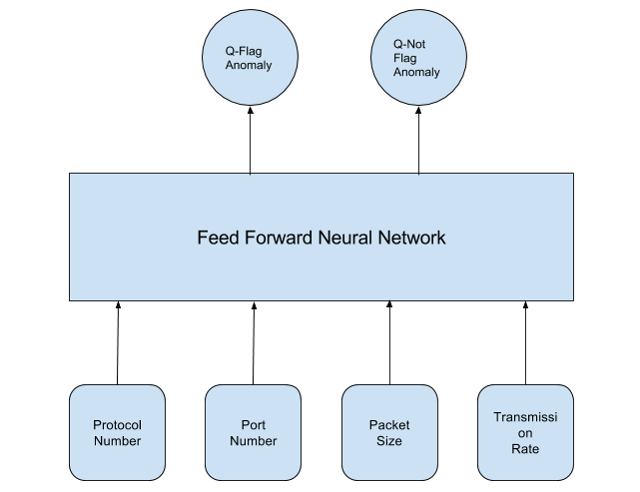
As an example of using reinforcement learning for anomaly detection, let us look at the well studied problem of network intrusion detection by finding anomalous behavior in network traffic flow⁷. For this purpose, one can use network flow parameters such as type of protocol (TCP, UDP), port number, packet size and rate of transmission as state variables. The action could be flag or not-flag an anomaly detection warning . We can use the following architecture for reinforcement learning of network intrusion.

Simulation of the Environment

As we mentioned earlier, in reinforcement learning, an agent interacts with an environment and takes actions on the current state. In return, the environment then supplies a new state and reward for the action taken by the agent. Therefore, we also need to create an environment to simulate a Network Intrusion Detection scenario. For this purpose we use the Gym Toolkit⁸ provided by the OpenAI foundation⁹.

We also use a standard dataset used for research purposes, for simulating this environment. This dataset, known as NSL-KDD dataset⁸, contains four categories of attacks. These are, Denial-of-Service (DoS) attack which floods a host website with a huge number of requests to make it slow; Remote-to-Local (R2L) attack where a remote hacker tries to get local user privileges; User-to-Root (U2R) attack where a hacker operates as a normal user and exploits vulnerabilities in the system; and the Probing attack where a hacker scans the machine to determine vulnerabilities which could be exploited later. Totally there are 148, 516 connections of which 53.5% are normal and the rest are malicious. The dataset contains 41 features of which 32 are continuous, 6 are binary and 3 are categorical. For the purpose of this study, we converted all the continuous features into categorical using binning, and then converted all the categorical variables to a binary representation using one hot encoding. These would be the states used as input to the DNN and in the environment for reinforcement learning.

A simple environment was created using the OpenAI Gym and NSL-KDD dataset, where the goal is to teach an autonomous agent to flag malicious network connection requests as anomalous. This is done by providing a positive reward of +1 when the agent makes correct actions (flag malicious network connection requests and do not flag normal connection requests) and a negative reward of -1 when the agent makes wrong actions (either flag normal connection requests or do not flag malicious connection requests).

Implementation of the Learning Process

In the Network Intrusion Detection scenario, the autonomous agent learns the optimal policies to flag a connection request as follows:

1. Initialize all the weights in DNN with random values.
2. Initialize the total accumulated reward to zero.
3. Get an initial state from the environment created using the OpenAI Gym and NSL-KDD dataset.
4. Repeat many episodes of learning, wherein each episode performs a series of explorations of the environment as follows:
   1. Start with the state obtained in the previous step.
   2. Perform a feed forward of the current state using DNN, and get the predicted Q(s, a) values.
   3. Take an action of either flag or not flag from the current state, according to the Q(s, a) values given by the output of the DNN in the previous state and in an ε-greedy manner.
   4. Get the reward and next state from the environment.
   5. Pass the new state also through the DNN, to compute the target Q(s, a) values using the Bellman’s equation.
   6. Perform a training of the DNN by back propagation of the error of prediction, where the difference between target Q(s, a) and predicted Q(s, a) in step 4.2 is taken as the error of prediction.
   7. Compute the new cumulative total reward.
   8. Repeat steps 4.1 to 4.7 for a finite number of explorations.

Once enough episodes of exploration are completed, the DNN would have adjusted its weights to predict correct Q(s, a) values, so that the agent would be able to act with optimal policies in any given state. The DNN model to learn Q(s, a) values is implemented using TensorFlow. Details of the implementation and results would be published in part 2 of this blog series.

References:

1. Artificial intelligence cyber attacks are coming-but what does it mean? blog post by Jeremy Straub, The Conversation https://theconversation.com/artificial-intelligence-cyber-attacks-are-coming-but-what-does-that-mean-82035
2. Anomaly Detection: A Survey,V. Chandole, A. Banerjee and V. Kumar, ACM Computing Surveys, CSUR, (2009)
3. Learning Intrusion Detection: Supervised or Unsupervised?, P. Laskov, P. Dussel, C. Schafer, K. Rieck, Proc. ICIAP 2005, September. Lecture Notes in Computer Science, LNCS 3617 (2005) 50-57
4. Next Generation Intrusion Detection: Autonomous Reinforcement Learning of Network Attacks, J. Cannadey, 23rd National Information Systems Security Conference (2000)
5. Sequential anomaly detection based on temporal-difference learning: Principles,
   models and case studies, Xin Xu, Applied Soft Computing 10 (2010) 859–867
6. Demystifying Deep Reinforcement Learning, Computational Neuroscience Lab blog, University of Tartu
   Towards Traffic Anomaly Detection via Reinforcement Learning and Data Flow, A. Servin
7. Open AI Gym Toolkit https://github.com/openai/gym
8. Open AI Foundation https://openai.com/
9. NSL-KDD dataset, Canadian Institute for Cyber Security, University of New Brunswick, (http://www.unb.ca/cic/datasets/nsl.html)

Acknowledgements:
I would like to thank our CEO Deepak Dutt for constant encouragement to publish this blog and Hari Acharya, Prathyusha Venugopal for critical reading of the manuscript.